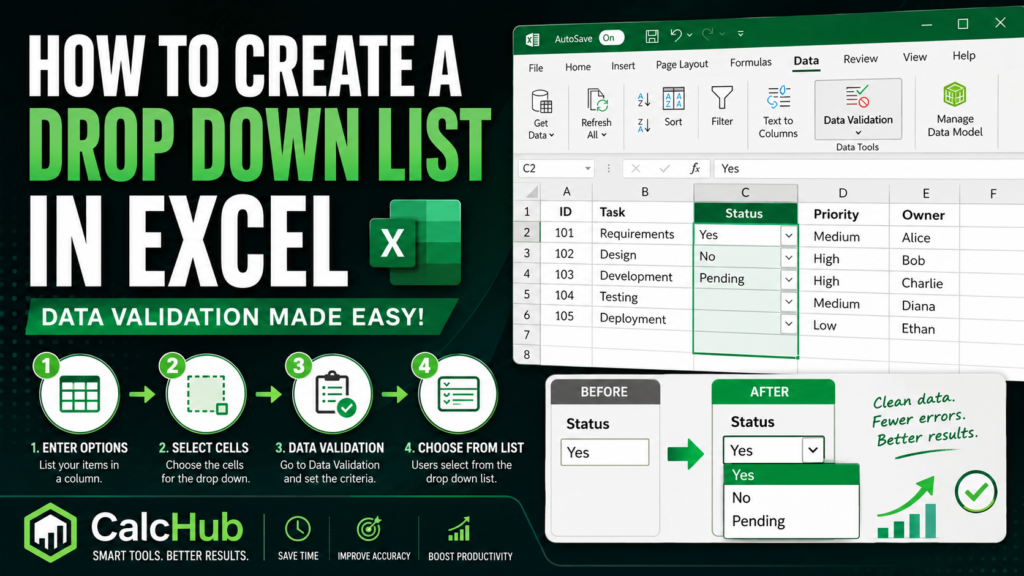
Want to add a drop down list in Excel? It is easy to do. A drop down lets users pick from a list instead of typing. So data stays clean and correct. This guide shows you three ways to create one. Follow the steps and you will be done in minutes.
What Is a Drop Down List in Excel?
A drop down list is a cell with a small arrow. You click the arrow and a list shows up. Then you pick one item. It goes straight into the cell.
People use drop downs for many things. Here are some good examples:
- Task status — Done, In Progress, Not Started
- Department — Sales, HR, Finance, IT
- Rating — 1, 2, 3, 4, 5
- Simple answer — Yes or No
- Country or city names
Drop downs are great because they stop typing errors. They also make data entry much faster. So your spreadsheet stays clean and easy to read.
Drop down lists are part of a feature called Data Validation. You can find it in the Data tab. It controls what a user can type or pick in a cell.
Method 1 — Type Your Own Items
This is the quickest way to make a drop down. You simply type the list items yourself. It works best for short lists that do not change. For example, Yes and No, or a set of status labels.
Follow These Steps
Click on the cell where the drop down should go. You can also select many cells at once. For example, click C2 and drag down to C50. Then the drop down will apply to all of them.
| A | B | C | |
|---|---|---|---|
| 1 | Task | Owner | Status |
| 2 | Write report | Ali | ← click here |
| 3 | Send email | Sara | |
| 4 | Review file | Ahmed |
Go to the Data tab. Then click Data Validation. A box will open on screen.
Data Tools→
Data Validation
In the box, click the Allow field. Then choose List from the menu. A Source field will appear below it.
Click in the Source box. Then type your items. Put a comma between each one. Do not add spaces after the commas.
// Use commas to split each item
Click OK. Go back to your cell. You will see a small arrow on the right. Click it and the list appears. Pick an item and it fills the cell.
Before you open Data Validation, select all the cells you need. For instance, select C2 to C100. Then follow the steps. As a result, all cells get the drop down at once. You do not have to repeat the steps.
Method 2 — Use a Cell Range
This method is better for longer lists. Instead of typing items in the Source box, you put them in a column. Then you point the drop down to that column.
This way is easier to manage. For example, to add a new item, you just type it in the column. You do not need to open Data Validation again.
Step One — Put Your Items in a Column
Type your list in a column. A separate sheet is a good place for this. Put one item per row. Start from the top.
| A | |
|---|---|
| 1 | Department |
| 2 | Sales |
| 3 | HR |
| 4 | Finance |
| 5 | IT |
| 6 | Operations |
Step Two — Open Data Validation
Go to your main sheet. Click the cell for the drop down. Then open Data Validation the same way as before.
Data Tools→
Data Validation
Step Three — Point to Your Range
Set Allow to List. Then click the Source box. Go to your list column and select the cells. Or type the range yourself.
=$A$2:$A$6
// From a sheet called “Lists”:
=Lists!$A$2:$A$6
Then click OK. Your drop down will now show all items from that column. To add a new option later, just type it in the column. The drop down picks it up right away.
Always use dollar signs when typing the range. For example, write $A$2:$A$6 and not A2:A6. This keeps the range fixed. So the drop down still works when you copy it to other cells.
Method 3 — Dynamic Drop Down with an Excel Table
This is the best method for lists that change often. When you use a Table as the source, the drop down updates on its own. You add a row to the table and it appears in the list. You remove a row and it disappears. No extra steps needed.
Step One — Turn Your List into a Table
Select your list items. Then press Ctrl+T. Click OK. Excel turns it into a Table. Give the Table a name. For example, name it DeptList.
Ctrl + T→
Name the Table
Step Two — Set Up Data Validation with INDIRECT
Select your drop down cell. Open Data Validation. Set Allow to List. Then type this in the Source box:
// DeptList = name of your Table
// Department = name of the column header
Step Three — Click OK
Click OK. From now on, the drop down updates itself. Add a new row to the Table and it shows in the list. Remove a row and it is gone. You never need to open Data Validation again.
Just edit the Table and the drop down updates on its own.
Which Method Is Best for You?
All three methods work well. The right one depends on what you need. Here is a simple guide to help you choose.
Type Your Items
Good for short fixed lists. For example, Yes or No. Quick to set up.
Use a Cell Range
Good for longer lists. Easy to update in one place. No need to reopen settings.
Use a Table
Best for lists that change. Fully automatic. The drop down updates itself.
Our Pick
Use Method 3 for real projects. Use Method 1 for quick one-off tasks.
How to Edit or Delete a Drop Down List
How to Change the Items
Click the cell with the drop down. Then go to Data Validation. Change the Source field and click OK. The list will update right away.
But if your source is a cell range, just edit the cells in that column. You do not need to open Data Validation at all. The drop down picks up the changes on its own.
How to Remove the Drop Down
Click the cell. Then open Data Validation. Click Clear All in the bottom left. Then click OK. The cell goes back to normal. It is now a plain cell with no rules.
Select all the cells that have the drop down. Then open Data Validation and click Clear All. So all selected cells lose the drop down in one step. Much faster than doing them one by one.
How to Copy a Drop Down to Other Cells
You do not need to set up Data Validation for every cell. Instead, you can copy the drop down very fast. Here is how to do it.
Click the cell that has the drop down. Then press Ctrl+C to copy it.
Now select all the cells where you want the same drop down.
Right-click on the selected cells. Then choose Paste Special. Select Validation and click OK. Only the drop down rule is pasted. The cell value and format do not change.
Paste Special→
Validation → OK
Useful Tips for Drop Down Lists
Show a Hint When Someone Clicks the Cell
Open Data Validation. Go to the Input Message tab. Turn it on. Then type a short message. For example: “Pick a status from the list.” So users know what to do when they click the cell.
Block Wrong Values
By default, users can still type values not in the list. But you can block this. Open Data Validation. Go to the Error Alert tab. Turn it on. Set the style to Stop. Then type a message. Now Excel blocks any wrong entry and shows your message instead.
Make Drop Down Cells Easy to See
Add a light background color to cells with a drop down. Go to Home tab and click Fill Color. Pick a soft color like light blue. So users can spot the drop down cells at a glance.
Quick Reference Table
| What You Want to Do | How to Do It |
|---|---|
| Add a drop down | Data tab → Data Validation → Allow: List |
| Change the items | Click cell → Data Validation → edit Source → OK |
| Remove the drop down | Data Validation → Clear All → OK |
| Copy to other cells | Copy → Paste Special → Validation |
| Block wrong values | Data Validation → Error Alert → Stop |
| Show a hint | Data Validation → Input Message → type hint |
Frequently Asked Questions
Click the cell you want. Then go to the Data tab and click Data Validation. Set Allow to List. Type your items in the Source box and put a comma between each one. Then click OK. That is it — the drop down is ready to use.
Yes, you can. Put your items on a separate sheet. Then in the Source box, type the sheet name and the range. For example, type =Lists!$A$2:$A$10. Replace Lists with your sheet name. So your list items stay separate from your main data.
If you typed the items in the Source box, open Data Validation and change them there. But if your source is a cell range, just edit the cells in that column. The drop down will update on its own. No need to open Data Validation again.
Click the cell. Then open Data Validation from the Data tab. Click Clear All in the bottom left corner. Then click OK. The drop down is gone and the cell is normal again. To remove it from many cells, select them all first and then follow the same steps.
Open Data Validation. Go to the Error Alert tab. Turn it on. Set the style to Stop. Then type a short message. From now on, Excel will block any value that is not in the list. It will show your message to the user instead.
Turn your list into an Excel Table first. Select the list and press Ctrl+T. Give the Table a name. Then in the Data Validation Source box, use this formula: =INDIRECT(“TableName[ColumnName]”). Now when you add or remove rows in the Table, the drop down updates on its own.
Yes. Copy the cell with the drop down using Ctrl+C. Then select all target cells. Right-click and choose Paste Special. Then pick Validation and click OK. Only the drop down rule is copied. The cell value and format stay the same.
Need a Free Calculator Too?
CalcHub has free tools for percentage, BMI, age, loan, and more. No sign-up. Works on any device.